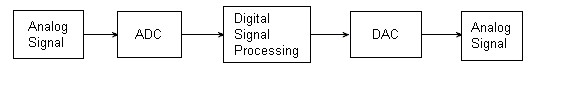
Digital signal processing is often implemented using specialised microprocessors such as the DSP56000, the TMS320, or the SHARC. These often process data using fixed-point arithmetic, although some versions are available which use floating point arithmetic and are more powerful. For faster applications FPGAs might be used. Beginning in 2007, multicore implementations of DSPs have started to emerge from companies including Freescale and Stream Processors, Inc. For faster applications with vast usage, ASICs might be designed specifically. For slow applications, a traditional slower processor such as a microcontroller may be adequate.

The Digital Signal Processor (DSP) measures or filter continuous analog signals in real-time. Analog signals are sampled and converted to digital form by an analog-to-digital converter (ADC), manipulated digitally, and then converted again to analog form with a digital-to-analog (DAC).

Signal sampling

A digital signal is often a numerical representation of a continuous signal. This discrete representation of a continuous signal will generally introduce some error in to the data. The accuracy of the representation is mostly dependent on two things; sampling frequency and the number of bits used for the representation. The continuous signal is usually sampled at regular intervals and the value of the continuous signal in that interval is represented by a discrete value. The sampling frequency or sampling rate is then the rate at which new samples are taken from the continuous signal. The number of bits used for one value of the discrete signal tells us how accurately the signal magnitude is represented. Similarly, the sampling frequency controls the temporal or spatial accuracy of the discrete signal.

Sampling is usually carried out in two stages, discretization and quantization. In the discretization stage, the space of signals is partitioned into equivalence classes and quantization is carried out by replacing the signal with representative signal of the corresponding equivalence class. In the quantization stage the representative signal values are approximated by values from a finite set.

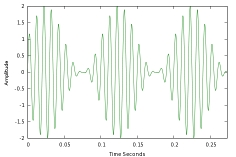
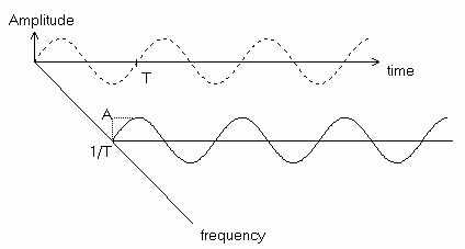
There are many kinds of signal processors, each one of them being better suited for a specific task. And not all DSPs provide the same speed. Generally, DSPs are dedicated RISC processors, however DSP functionality can also be realized using Field Programmable Gate Array (FPGA) chips.

DSPs use algorithms to process signals in one of the following domains: time domain, frequency domain (one-dimensional signals), spatial domain (multidimensional signals), autocorrelation domain, and wavelet domains. Which domain to chose depends on the essential characteristic of the signal. A sequence of samples from a measuring device produces a time or spatial domain representation, whereas a discrete Fourier transform produces the frequency domain information, that is the frequency spectrum. Autocorrelation is defined as the cross-correlation of the signal with itself over varying intervals of time or space.

Time Domain vs Frequency Domain

A time domain graph shows how a signal changes over time, whereas a frequency domain graph shows how much of the signal lies within each given frequency band over a range of frequencies. The time - amplitude axes on which the signalis shown define the time plane. Time domain signals are measured with an oscilloscope and frequency domain signals are measured with a spectrometer.

The basic idea of signal processing is that a complex, time-domain waveform like this —

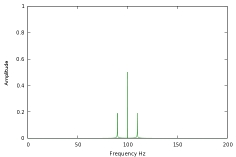
— can be fully and completely recreated using a frequency-domain representation like this:

If a frequency domain axis is added to the time domain axis, then the signal would be as illustrated below.

Over 80% of all DSP applications require some form of frequency domain processing and there are many techniques for performing this kind of operation.

Spatial Domain vs Frequency Domain

Audio signals are dealt with in the frequency domain, while image signals are handled in the spatial domain.

An image also can be thought of as a collection of spatial signals. From signal processing, we know that any signal can be reduced, or decomposed, into a series of simple sinusoidal components, each of which has a frequency, amplitude, and phase. As such, it is possible to change, or transform, an image from the spatial domain into the frequency domain. In the frequency domain image information is represented as signals having various amplitute, frequency and phase characteristics. Some frequency-based operations, such as high-pass, low-pass, and band-pass filtering, can be performed easily on a frequency domain image, while the equivalent operation in the spatial domain involves cumbersome and time-consuming convolutions. In addition, the accuracy of frequency oriented operations are often higher than if they were performed in the spatial domain.

As an example, consider the use of frequency domain processing for filtering. In the first image shown below, there is a distinct repetitive diagonal noise pattern that runs primarily from the upper right to lower left. In addition, there is a more subtle pattern running from the upper left to lower right. The FFT of this image is shown next. This is a typical example of an image's power spectra. The four bright, off-axis spots represent the unwanted noise. (Remember, each frequency has an identical but negative component.)

At this point, the power of filtering in the frequency domain becomes apparent. The noise can be eliminated by simply removing the unwanted frequency components from the power spectra. The next image shows the necessary modification that eliminates the noise. Now all that is needed is to perform the inverse FFT, returning the image to the spatial domain. The last image in this set shows the result. As can be seen, nearly all of the noise is gone. This same procedure can be invoked to perform high-pass filtering (eliminating the low frequencies clustered near the center of the power spectra) or low-pass filtering (eliminating all but the central low frequencies). It might seem to be a lot of trouble to perform frequency operations that could be performed in the spatial domain with convolution, but operating in the frequency domain affords more control and may be required for certain applications.

Time and spatial domains filtering

The most common processing approach in the time or spatial domain is enhancement of the input signal through a method called filtering. Filtering generally consists of some transformation of a number of surrounding samples around the current sample of the input or output signal.

Properties such as the following characterize filters:

			A "linear" filter consists of a linear transformation of input samples; other filters are "non-linear." Linear filters satisfy the superposition condition, i.e. if an input signal is a weighted linear combination of different input signals, the output will be an equally weighted linear combination of the corresponding individual output signals.
			A "causal" transformation uses only previous samples of the input or output signals; transformations that also use future input samples are "non- causal." Adding a delay will transform many non-causal filters into causal filters.
			A "time-invariant" filter has constant properties over time; other filters such as adaptive filters change in time.
			"Finite impulse response" (FIR) filters use only the input signal; so-called "infinite impulse response" filters use both the input signal and previous samples of the output signal.

Most filters can be described by their Transfer functions.

Contact email: qooljaq@qooljaq.com